本文记录线性代数学习中的向量绘图示例,结合代码、逐行说明与截图展示绘图过程。
绘制箭头图
quiver 用一组箭头表示二维向量场。这个例子在每个网格点 (x, y) 放置一个分量为 (x, y) 的向量,画出来的箭头从原点向四周散开。
完整代码
import matplotlib.pyplot as plt
import numpy as np

X = np.arange(-10, 10, 1)
Y = np.arange(-10, 10, 1)
U, V = np.meshgrid(X, Y)

fig, ax = plt.subplots()
q = ax.quiver(X, Y, U, V)
ax.quiverkey(q, X=0.3, Y=1.1, U=10,
             label='Quiver key, length = 10', labelpos='E')

plt.show()
逐行理解
| 代码 | 作用 |
|---|---|
import matplotlib.pyplot as plt |
导入绘图接口,简写为 plt。 |
import numpy as np |
导入 NumPy,简写为 np,用于创建数组和网格。 |
X = np.arange(-10, 10, 1) |
生成横坐标,从 -10 到 9,共 20 个。 |
Y = np.arange(-10, 10, 1) |
生成纵坐标,也有 20 个。横纵坐标组合成 400 个网格点。 |
U, V = np.meshgrid(X, Y) |
将两个一维数组展开成两个 (20, 20) 的矩阵,这里直接用作水平和竖直分量。 |
fig, ax = plt.subplots() |
创建整张图 fig 和其中的绘图区 ax。 |
q = ax.quiver(X, Y, U, V) |
在网格点上绘制箭头,返回的 q 代表这组箭头。 |
ax.quiverkey(...) |
为 q 添加一支表示向量大小为 10 的参考箭头。 |
plt.show() |
显示图形。 |
为什么 quiver 要传四组值?
一支箭头需要两组数据。X, Y 决定箭尾的位置,U, V 决定向量的水平和竖直分量。 固定箭尾在 (3, -4) 时,分量 (3, -4) 让箭头朝右下,分量 (0, 1) 则让它朝上。
在本例中,X, Y 是一维坐标数组,U, V 是二维矩阵。Matplotlib 会用 X, Y 展开位置网格,再按行列配对。第 i 行、第 j 列对应的箭尾是 (X[j], Y[i]),分量是 (U[i, j], V[i, j])。因此,分量矩阵的形状是 (len(Y), len(X))。
用两行三列的小网格看这个对应关系:
X = np.array([2, 5, 8])
Y = np.array([-1, 3])
U, V = np.meshgrid(X, Y)

# U = [[ 2,  5,  8],
#      [ 2,  5,  8]]
#
# V = [[-1, -1, -1],
#      [ 3,  3,  3]]
取第 0 行、第 1 列,箭尾是 (X[1], Y[0]) = (5, -1),向量分量是 (U[0, 1], V[0, 1]) = (5, -1),所以箭头朝右下。位置和分量恰好相同,是因为这段代码把网格坐标直接赋给了 U, V。
图形长什么样?
从原图中挑 9 个网格点,示意如下:
              x = -4     x = 0     x = 4

y =  4           ↖         ↑         ↗
y =  0           ←         ·         →
y = -4           ↙         ↓         ↘
原点的分量是 (0, 0),图中用点表示零向量。其余位置的向量沿着从原点到该位置的方向向外。向量大小为 sqrt(x**2 + y**2),所以越远离原点,向量越大。例如 (4, 0) 和 (8, 0) 的箭头都朝右,向量大小分别为 4 和 8。Matplotlib 默认会自动缩放箭头的显示长度。
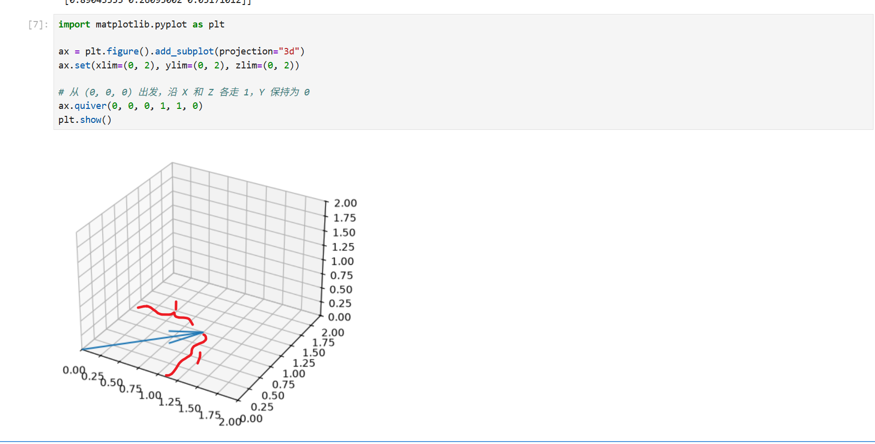
你可以先在 Notebook 里画一支箭头,再回来看网格版:
import matplotlib.pyplot as plt

ax = plt.figure().add_subplot(projection="3d")
ax.set(xlim=(0, 2), ylim=(0, 2), zlim=(0, 2))

# 从 (0, 0, 0) 出发,沿 X 和 Z 各走 1,Y 保持为 0
ax.quiver(0, 0, 0, 1, 1, 0)
plt.show()
绘制平面散点图
散点图用一个点表示一条观测。横坐标和纵坐标分别对应两个变量,便于观察它们的关系。例如,可以把学习时长放在横轴,把分数放在纵轴。
1. 直接传入坐标
import matplotlib.pyplot as plt
import seaborn as sns

hours = [1, 2, 3, 4, 5]
scores = [58, 65, 63, 78, 85]

ax = sns.scatterplot(x=hours, y=scores)
ax.set(xlabel="Study hours", ylabel="Score")
plt.show()
x=hours指定横坐标,y=scores指定纵坐标。两个列表长度相同,按索引配对,依次得到(1, 58)、(2, 65)、(3, 63)等点。sns.scatterplot()返回 Matplotlib 的绘图区对象ax。这里用ax.set()设置轴标签。plt.show()显示图形。
这组数据的分数整体随学习时长上升,不过从 2 小时到 3 小时,分数从 65 降到 63。散点图能同时看出整体趋势和单个观测的差异。
2. 用 DataFrame 指定列,按组着色
import matplotlib.pyplot as plt
import pandas as pd
import seaborn as sns

df = pd.DataFrame({
    "hours": [1, 2, 3, 4, 5],
    "score": [58, 65, 63, 78, 85],
    "group": ["A", "B", "A", "B", "A"],
})

ax = sns.scatterplot(data=df, x="hours", y="score", hue="group")
ax.set(xlabel="Study hours", ylabel="Score")
plt.show()
data=df 提供表格,x="hours" 和 y="score" 指定列名。表格的每一行对应一个点。例如,第一行的 hours=1、score=58、group="A" 会在 (1, 58) 画一个 A 组颜色的点。加上 hue="group" 后,A、B 两组的颜色会显示在图例里。
3. 常用参数
| 参数 | 控制什么 | 示例 |
|---|---|---|
x、y |
点的横纵位置 | x="hours", y="score" |
hue |
按变量映射颜色 | hue="group" |
style |
按类别映射点的形状 | style="group" |
size |
按变量映射点的面积 | size="hours" |
s |
给所有点设置相同的面积,单位为平方磅 | s=80 |
alpha |
点的透明度,取值为 0 到 1 | alpha=0.6 |
ax |
指定绘图所在的 Matplotlib 绘图区 | ax=ax |
在分组例子里,可以同时传入 hue="group" 和 style="group",让 A、B 两组同时通过颜色和形状区分。如果只想把所有点统一调大,用 s=80 即可。
绘制三维散点图
import matplotlib.pyplot as plt
import numpy as np

# Fixing random state for reproducibility
np.random.seed(19680801)


def randrange(n, vmin, vmax):
    """
    Helper function to make an array of random numbers having shape (n, )
    with each number distributed Uniform(vmin, vmax).
    """
    return (vmax - vmin)*np.random.rand(n) + vmin

fig = plt.figure()
ax = fig.add_subplot(projection='3d')

n = 100

# For each set of style and range settings, plot n random points in the box
# defined by x in [23, 32], y in [0, 100], z in [zlow, zhigh].
for m, zlow, zhigh in [('o', -50, -25), ('^', -30, -5)]:
    xs = randrange(n, 23, 32)
    ys = randrange(n, 0, 100)
    zs = randrange(n, zlow, zhigh)
    ax.scatter(xs, ys, zs, marker=m)

ax.set_xlabel('X Label')
ax.set_ylabel('Y Label')
ax.set_zlabel('Z Label')

plt.show()
绘制向量图
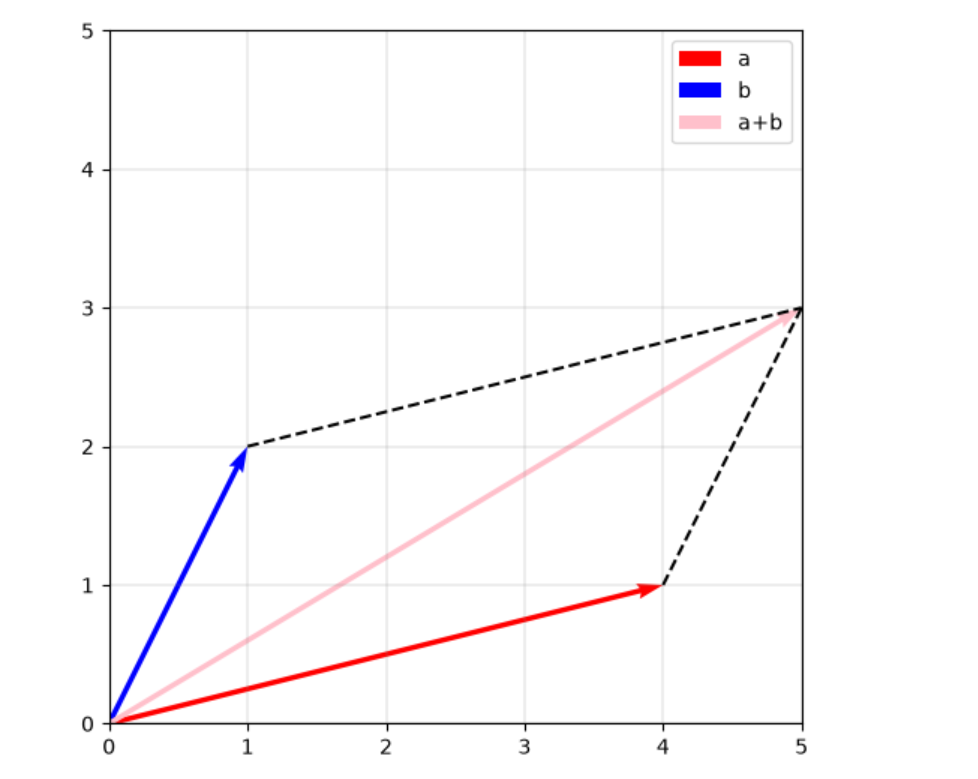
a+b
import matplotlib.pyplot as plt
import numpy as np

a_vec = np.array([4,1])
b_vec = np.array([1,2])

a_p_b_vec = a_vec + b_vec

plt.figure(figsize=(6,6))
plt.quiver(0,0,a_vec[0],a_vec[1],angles='xy',scale_units='xy',scale=1,color='r',label="a")
plt.quiver(0,0,b_vec[0],b_vec[1],angles='xy',scale_units='xy',scale=1,color='b',label="b")

plt.quiver(0,0,a_p_b_vec[0],a_p_b_vec[1],angles='xy',scale_units='xy',scale=1,color='pink',label="a+b")

#k-- 表示黑色虚线
plt.plot([b_vec[0],a_p_b_vec[0]],[b_vec[1],a_p_b_vec[1]],'k--')
plt.plot([a_vec[0],a_p_b_vec[0]],[a_vec[1],a_p_b_vec[1]],'k--')

#equal 让 x 轴上的 1 个单位和 y 轴上的 1 个单位在图上等长
# box 通过调整绘图区的宽高来满足这个比例
plt.gca().set_aspect('equal', adjustable='box')

#分别把横轴、纵轴的显示范围设为 0 到 5
plt.xlim(0, 5)
plt.ylim(0, 5)

#在y=0 x=0画一条贯穿绘图区的黑色水平线。
plt.axhline(0, color='black', linewidth=0.5)
plt.axvline(0, color='black', linewidth=0.5)

#显示网格。`color='gray' 设为灰色,alpha=0.8` 设置不透明度,`linestyle='-' 使用实线,linewidth=0.25` 设置线宽为 0.25 磅
plt.grid(color='gray', alpha=0.8, linestyle='-', linewidth=0.25)

#读取前面三次 plt.quiver() 的 label,显示 a、`b`、`a+b` 的图例。
plt.legend()